2. General lattice attributes
After configuring the lattice the general attributes and methods are available.
Even without building a (finite) lattice structure all properties can be computed on
the fly for a given lattice vector, consisting of the translation vector n and
the index alpha of the atom in the unit cell.
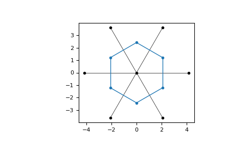
We will discuss all properties with a simple hexagonal lattice as example:
>>> latt = lp.Lattice.hexagonal()
>>> latt.add_atom()
>>> latt.add_connections()
>>> latt.plot_cell()
>>> plt.show()
2.1. Unit cell properties
The basis vectors of the lattice can be accessed via the vectors property:
>>> latt.vectors
[[ 1.5        0.8660254]
 [ 1.5       -0.8660254]]
The size and volume of the unit cell defined by the basis vectors are also available:
>>> latt.cell_size
[1.5        1.73205081]
>>> latt.cell_volume
2.598076211353316
The results are all computed in cartesian corrdinates.
2.2. Transformations and atom positions
Coordinates in cartesian coordinates (also referred to as world coordinates) can be tranformed to the lattice or basis coordinate system and vice versa. Consider the point \(\boldsymbol{n} = (n_1, \dots, n_d)\) in the basis coordinate system, which can be understood as a translation vector. The point \(\boldsymbol{x} = (x_1, \dots, x_d)\) in cartesian coordinates then is given by
>>> n = [1, 0]
>>> x = latt.transform(n)
>>> x
[1.5       0.8660254]
>>> latt.itransform(x)
[1. 0.]
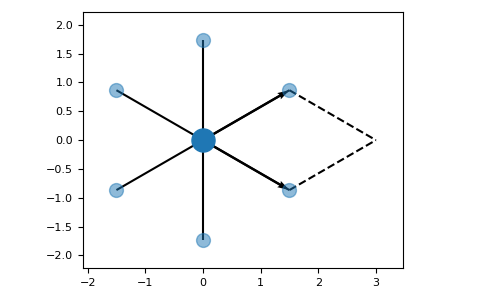
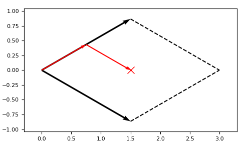
The points in the world coordinate system do not have to match the lattice points defined by the basis vectors:
>>> latt.itransform([1.5, 0.0])
[0.5 0.5]
latt = lp.Lattice.hexagonal() ax = latt.plot_cell()
ax.plot([1.5], [0.0], marker=”x”, color=”r”, ms=10) lp.plotting.draw_arrows(ax, 0.5 * latt.vectors[0], color=”r”, width=0.005) lp.plotting.draw_arrows(ax, [0.5 * latt.vectors[1]], pos=[0.5 * latt.vectors[0]], color=”r”, width=0.005) plt.show()

Both methods are vectorized and support multiple points as inputs:
>>> n = [[0, 0] [1, 0], [2, 0]]
>>> x = latt.transform(n)
>>> x
[[0.         0.        ]
 [1.5        0.8660254 ]
 [3.         1.73205081]]
>>> latt.itransform(x)
[[ 0.00000000e+00  0.00000000e+00]
 [ 1.00000000e+00 -3.82105486e-17]
 [ 2.00000000e+00 -7.64210971e-17]]
Note
As can be seen in the last example, some inaccuracies can occur in the transformations depending on the data type due to machine precision.
Any point \(\boldsymbol{r}\) in the cartesian cooridnates can be translated by a translation vector \(\boldsymbol{n} = (n_1, \dots, n_d)\):
The inverse operation is also available. It returns the translation vector \(\boldsymbol{n} = (n_1, \dots, n_d)\) and the point \(\boldsymbol{r}\) such that \(\boldsymbol{r}\) is the neareast possible point to the origin:
>>> n = [1, 0]
>>> r = [0.5, 0.0]
>>> x = latt.translate(n, r)
>>> x
[2.        0.8660254]
>>> latt.itransform(x)
(array([1, 0]), array([0.5, 0. ]))
Again, both methods are vectorized:
>>> n = [[0, 0], [1, 0], [2, 0]]
>>> r = [0.5, 0]
>>> x = latt.translate(n, r)
>>> x
[[0.5        0.        ]
 [2.         0.8660254 ]
 [3.5        1.73205081]]
>>> n2, r2 = latt.itranslate(x)
>>> n2
[[0 0]
 [1 0]
 [2 0]]
>>> r2
[[0.5 0. ]
 [0.5 0. ]
 [0.5 0. ]]
Specifiying the index of the atom in the unit cell alpha the positions of a
translated atom can be obtained via the translation vector \(\boldsymbol{n}\):
>>> latt.get_position([0, 0], alpha=0)
[0. 0.]
>>> latt.get_position([1, 0], alpha=0)
[1.5       0.8660254]
>>> latt.get_position([2, 0], alpha=0)
[3.         1.73205081]
Multiple positions can be computed by the get_positions method. The argument is
a list of lattice indices, consisting of the translation vector n and the atom index
alpha as a single array. Note the last column of indices in the following
example, where all atom indices alpha=0:
>>> indices = [[0, 0, 0], [1, 0, 0], [2, 0, 0]]
>>> latt.get_positions(indices)
[[0.         0.        ]
 [1.5        0.8660254 ]
 [3.         1.73205081]]
2.3. Neighbors
The maximal number of neighbors of the atoms in the unit cell for all distance levels
can be accessed by the property num_neighbors:
>>> latt.num_neighbors
[6]
Since the lattice only contains one atom in the unit cell a array with one element is returned. Similar to the position of a lattice site, the neighbors of a site can be obatined by the translation vector of the unit cell and the atom index. Additionaly, the distance level has to be specified via an index. The nearest neighbors of the site at the origin can, for example, be computed by calling
>>> neighbors = latt.get_neighbors([1, 0], alpha=0, distidx=0)
>>> neighbors
[[ 2 -1  0]
 [ 0  1  0]
 [ 0  0  0]
 [ 2  0  0]
 [ 1 -1  0]
 [ 1  1  0]]
The results ara again arrays cvontaining translation vectors plus the atom index alpha:
>>> neighbor = neighbors[0]
>>> n, alpha = neighbor[:-1], neighbor[-1]
>>> n
[ 2 -1]
>>> alpha
0
In addition to the lattice indices the positions of the neighbors can be computed:
>>> latt.get_neighbor_positions([1, 0], alpha=0, distidx=0)
[[ 1.5         2.59807621]
 [ 1.5        -0.8660254 ]
 [ 0.          0.        ]
 [ 3.          1.73205081]
 [ 0.          1.73205081]
 [ 3.          0.        ]]
or the vectors from the site to the neighbors
>>> latt.get_neighbor_positions(alpha=0, distidx=0)
[[ 0.          1.73205081]
 [ 0.         -1.73205081]
 [-1.5        -0.8660254 ]
 [ 1.5         0.8660254 ]
 [-1.5         0.8660254 ]
 [ 1.5        -0.8660254 ]]
Here no translation vector is needed since the vectors from a site to it’s neighbors are translational invariant.
2.4. Reciprocal lattice
The reciprocal lattice vectors of the Lattice instance can be computed via
>>> latt.reciprocal_vectors()
[[ 2.0943951   3.62759873]
 [ 2.0943951  -3.62759873]]
Also, the reciprocal lattice can be constrcuted, which has the reciprocal vectors from the current lattice as basis vectors:
>>> rlatt = latt.reciprocal_lattice()
>>> rlatt.vectors
[[ 2.0943951   3.62759873]
 [ 2.0943951  -3.62759873]]
The reciprocal lattice can be used to construct the 1. Brillouin zone of a lattice, whcih is defined as the Wigner-Seitz cell of the reciprocal lattice:
>>> bz = rlatt.wigner_seitz_cell()
Additionally, a explicit method is available:
>>> bz = latt.brillouin_zone()
The 1. Brillouin zone can be visualized:
>>> latt = lp.Lattice.hexagonal()
>>> bz = latt.brillouin_zone()
>>> bz.draw()
>>> plt.show()