3. Finite lattice models
So far only abstract, infinite lattices have been discussed. In order to construct a finite sized model of the configured lattice structure we have to build the lattice.
3.1. Build geometries
By default, the shape passed to the build is used to create a box in cartesian
coordinates. Alternatively, the geometry can be constructed in the basis of the lattice
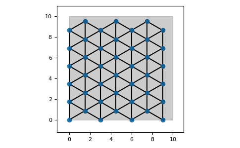
by setting primitive=True. As an example, consider the hexagonal lattice. We can
build the lattice in a box of the specified shape:
>>> latt = lp.Lattice.hexagonal()
>>> latt.add_atom()
>>> latt.add_connections()
>>> s = latt.build((10, 10))
>>> ax = latt.plot()
>>> s.plot(ax)
>>> plt.show()
or in the coordinate system of the lattice, which results in
>>> latt = lp.Lattice.hexagonal()
>>> latt.add_atom()
>>> latt.add_connections()
>>> s = latt.build((10, 10), primitive=True)
>>> ax = latt.plot()
>>> s.plot(ax)
>>> plt.show()

Other geometries can be build by using AbstractShape ojects:
>>> latt = lp.Lattice.hexagonal()
>>> latt.add_atom()
>>> latt.add_connections()
>>> s = lp.Circle((0, 0), radius=10)
>>> latt.build(s, primitive=True)
>>> ax = latt.plot()
>>> s.plot(ax)
>>> plt.show()
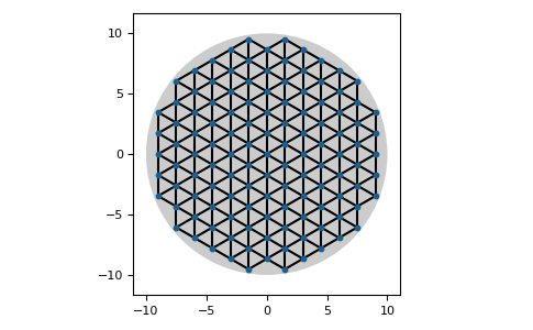

3.2. Periodic boundary conditions
After a finite size lattice model has been buildt periodic boundary conditions can be configured by specifying the axis of the periodic boundary conditions. The periodic boundary conditions can be set up for each axes individually, for example
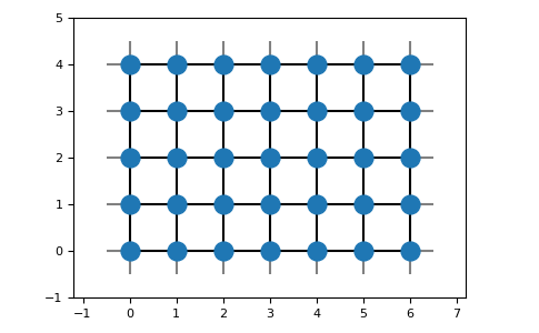
>>> latt = lp.simple_square()
>>> latt.build((6, 4))
>>> latt.set_periodic(0)
>>> latt.plot()
>>> plt.show()

or for multiple axes at once:
>>> latt = lp.simple_square()
>>> latt.build((6, 4))
>>> latt.set_periodic([0, 1])
>>> latt.plot()
>>> plt.show()

The periodic boundary conditions are computed in the same coordinate system chosen for
building the model. If primitive=False, i.e. world coordinates, the box around
the buildt lattice is repeated periodically:
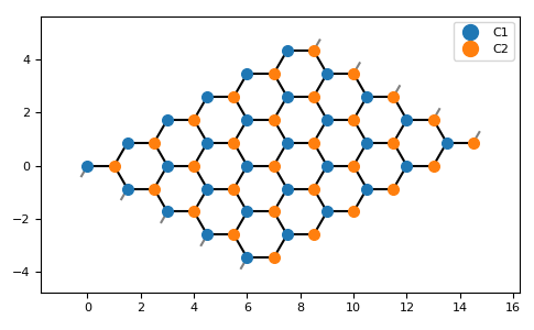
>>> latt = lp.graphene()
>>> latt.build((5.5, 4.5))
>>> latt.set_periodic(0)
>>> latt.plot()
>>> plt.show()
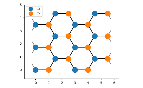

Here, the periodic boundary conditions again are set up along the x-axis, even though the basis vectors of the hexagonal lattice define a new basis. In the coordinate system of the lattice the periodic boundary contitions are set up along the basis vectors:
>>> latt = lp.graphene()
>>> latt.build((5.5, 4.5), primitive=True)
>>> latt.set_periodic(0)
>>> latt.plot()
>>> plt.show()

Warning
The set_periodic method assumes the lattice is build such that periodic
boundary condtitions are possible. This is especially important if a lattice
with multiple atoms in the unit cell is used. To correctly connect both sides of
the lattice it has to be ensured that each cell in the lattice is fully contained.
If, for example, the last unit cell in the x-direction is cut off in the middle
no perdiodic boundary conditions will be computed since the distance between the
two edges is larger than the other distances in the lattice.
A future version will check if this requirement is fulfilled, but until now the
user is responsible for the correct configuration.
3.3. Position and neighbor data
After building the lattice and optionally setting periodic boundary conditions the
information of the buildt lattice can be accessed. The data of the
lattice model then can be accessed by a simple index i. The syntax is the same as
before, just without the get_ prefix. In order to find the right index,
the plot method also supports showing the coorespnding super indices of the lattice sites:
>>> latt = lp.simple_square()
>>> latt.build((6, 4))
>>> latt.set_periodic(0)
>>> latt.plot(show_indices=True)
>>> plt.show()
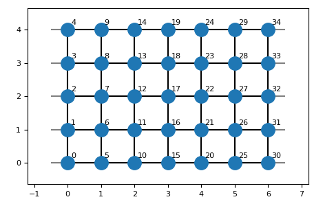
The positions of the sites in the model can now be accessed via the super index i:
>>> latt.position(2)
[0. 2.]
Similarly, the neighbors can be found via
>>> latt.neighbors(2, distidx=0)
[3 1 7 32]
The nearest neighbors also can be found with the helper method
>>> latt.nearest_neighbors(2)
[3 1 7 32]
The position and neighbor data of the finite lattice model is stored in the
LatticeData object, wich can be accessed via the data attribute.
Additionally, the positions and (lattice) indices of the model can be directly
fetched, for example
>>> latt.positions
[[0. 0.]
 [0. 1.]
 ...
 [6. 3.]
 [6. 4.]]
3.4. Data map
The lattice model makes it is easy to construct the (tight-binding) Hamiltonian of a non-interacting model:
>>> latt = simple_chain(a=1.0)
>>> latt.build(shape=4)
>>> n = latt.num_sites
>>> eps, t = 0., 1.
>>> ham = np.zeros((n, n))
>>> for i in range(n):
...     ham[i, i] = eps
...     for j in latt.nearest_neighbors(i):
...         ham[i, j] = t
>>> ham
[[0. 1. 0. 0. 0.]
 [1. 0. 1. 0. 0.]
 [0. 1. 0. 1. 0.]
 [0. 0. 1. 0. 1.]
 [0. 0. 0. 1. 0.]]
Since we loop over all sites of the lattice the construction of the hamiltonian is slow. An alternative way of mapping the lattice data to the hamiltonian is using the DataMap object returned by the map() method of the lattice data. This stores the atom-types, neighbor-pairs and corresponding distances of the lattice sites. Using the built-in masks the construction of the hamiltonian-data can be vectorized:
>>> from scipy import sparse
>>> eps, t = 0., 1.
>>> dmap = latt.data.map()               # Build datamap
>>> values = np.zeros(dmap.size)         # Initialize array for data of H
>>> values[dmap.onsite(alpha=0)] = eps   # Map onsite-energies to array
>>> values[dmap.hopping(distidx=0)] = t  # Map hopping-energies to array
>>> ham_s = sparse.csr_matrix((values, dmap.indices))
>>> ham_s.toarray()
[[0. 1. 0. 0. 0.]
 [1. 0. 1. 0. 0.]
 [0. 1. 0. 1. 0.]
 [0. 0. 1. 0. 1.]
 [0. 0. 0. 1. 0.]]