1. Configuration

The Lattice object of LattPy can be configured in a few steps. There are three fundamental steps to defining a new structure:

1. Defining basis vectors of the lattice

2. Adding atoms to the unit cell

3. Adding connections to neighbors

1.1. Basis vectors

The core of a Bravais lattice are the basis vectors \(\boldsymbol{A} = \boldsymbol{a}_i\) with \(i=1, \dots, d\), which define the unit cell of the lattice. Each lattice point is defined by a translation vector \(\boldsymbol{n} = (n_1, \dots, n_d)\):

\[\boldsymbol{R_n} = \sum_{i=1}^d n_i \boldsymbol{a}_i.\]

A new Lattice instance can be created by simply passing the basis vectors of the system. A one-dimensional lattice can be initialized by passing a scalar or an \(1 \times 1\) array to the Lattice constructor:

>>> latt = lp.Lattice(1.0)
>>> latt.vectors
[[1.0]]

For higher dimensional lattices an \(d \times d\) array with the basis vectors as rows,

\[\begin{split}\boldsymbol{A} = \begin{pmatrix} a_{11} & \dots & a_{1d} \\ \vdots & \ddots & \vdots \\ a_{d1} & \dots & a_{dd} \end{pmatrix},\end{split}\]

is expected. A square lattice, for example, can be initialized by a 2D identity matrix:

>>> latt = lp.Lattice(np.eye(2))
>>> latt.vectors
[[1. 0.]
 [0. 1.]]

The basis vectors of frequently used lattices can be intialized via the class-methods of the Lattice object, for example:

lattpy.Lattice.chain([a])	Initializes a one-dimensional lattice.
lattpy.Lattice.square([a])	Initializes a 2D lattice with square basis vectors.
lattpy.Lattice.rectangular([a1, a2])	Initializes a 2D lattice with rectangular basis vectors.
lattpy.Lattice.hexagonal([a])	Initializes a 2D lattice with hexagonal basis vectors.
lattpy.Lattice.oblique(alpha[, a1, a2])	Initializes a 2D lattice with oblique basis vectors.
lattpy.Lattice.hexagonal3d([a, az])	Initializes a 3D lattice with hexagonal basis vectors.
lattpy.Lattice.sc([a])	Initializes a 3D simple cubic lattice.
lattpy.Lattice.fcc([a])	Initializes a 3D face centered cubic lattice.
lattpy.Lattice.bcc([a])	Initializes a 3D body centered cubic lattice.

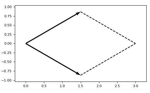
The resulting unit cell of the lattice can be visualized via the plot_cell() method:

>>> latt = lp.Lattice.hexagonal(a=1)
>>> latt.plot_cell()
>>> plt.show()

(png, pdf)

1.2. Adding atoms

Until now only the lattice type has been defined via the basis vectors. To define a lattice structure we also have to specify the basis of the lattice by adding atoms to the unit cell. The positions of the atoms in the lattice then are given by

\[\boldsymbol{R}_{n\alpha} = \boldsymbol{R_n} + \boldsymbol{r_\alpha},\]

where \(\boldsymbol{r_\mu}\) is the position of the atom \(\alpha\) relative to the origin of the unit cell.

In LattPy, atoms can be added to the Lattice object by calling add_atom() and supplying the position and type of the atom:

>>> latt = lp.Lattice.square()
>>> latt.add_atom([0.0, 0.0], "A")

If the position is omitted the atom is placed at the origin of the unit cell. The type of the atom can either be the name or an Atom instance:

>>> latt = lp.Lattice.square()
>>> latt.add_atom([0.0, 0.0], "A")
>>> latt.add_atom([0.5, 0.5], lp.Atom("B"))
>>> latt.atoms[0]
Atom(A, size=10, 0)
>>> latt.atoms[1]
Atom(B, size=10, 1)

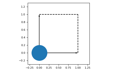
If a name is passed, a new Atom instance is created. We again can view the current state of the unit cell:

>>> latt = lp.Lattice.square()
>>> latt.add_atom([0.0, 0.0], "A")
>>> ax = latt.plot_cell()
>>> ax.set_xlim(-0.3, 1.3)
>>> ax.set_ylim(-0.3, 1.3)
>>> plt.show()

(png, pdf)

1.3. Adding connections

Finally, the connections of the atoms to theirs neighbors have to be set up. LattPy automatically connects the neighbors of sites up to a specified level of neighbor distances, i.e. nearest neighbors, next nearest neighbors and so on. The maximal neighbor distance can be configured for each pair of atoms independently. Assuming a square lattice with two atoms A and B in the unit cell, the connections between the A atoms can be set to next nearest neighbors, while the connections between A and B can be set to nearest neighbors only:

>>> latt = lp.Lattice.square()
>>> latt.add_atom([0.0, 0.0], "A")
>>> latt.add_atom([0.5, 0.5], "B")
>>> latt.add_connection("A", "A", 2)
>>> latt.add_connection("A", "B", 1)
>>> latt.analyze()

After setting up all the desired connections in the lattice the analyze method has to be called. This computes the actual neighbors for all configured distances of the atoms in the unit cell. Alternatively, the distances for all pairs of the sites in the unit cell can be configured at once by calling the add_connections method, which internally calls the analyze method. This speeds up the configuration of simple lattices.

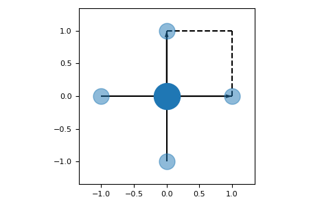
The final unit cell of the lattice, including the atoms and the neighbor information, can again be visualized:

>>> latt = lp.Lattice.square()
>>> latt.add_atom()
>>> latt.add_connections(1)
>>> latt.plot_cell()
>>> plt.show()

(png, pdf)