Quick-Start

A new instance of a lattice model is initialized using the unit-vectors of the Bravais lattice. After the initialization the atoms of the unit-cell need to be added. To finish the configuration the connections between the atoms in the lattice have to be set. This can either be done for each atom-pair individually by calling add_connection or for all possible pairs at once by callling add_connections. The argument is the number of unique distances of neighbors. Setting a value of 1 will compute only the nearest neighbors of the atom.

>>> import numpy as np
>>> from lattpy import Lattice
>>>
>>> latt = Lattice(np.eye(2))                 # Construct a Bravais lattice with square unit-vectors
>>> latt.add_atom(pos=[0.0, 0.0])             # Add an Atom to the unit cell of the lattice
>>> latt.add_connections(1)                   # Set the maximum number of distances between all atoms
>>>
>>> latt = Lattice(np.eye(2))                 # Construct a Bravais lattice with square unit-vectors
>>> latt.add_atom(pos=[0.0, 0.0], atom="A")   # Add an Atom to the unit cell of the lattice
>>> latt.add_atom(pos=[0.5, 0.5], atom="B")   # Add an Atom to the unit cell of the lattice
>>> latt.add_connection("A", "A", 1)          # Set the max number of distances between A and A
>>> latt.add_connection("A", "B", 1)          # Set the max number of distances between A and B
>>> latt.add_connection("B", "B", 1)          # Set the max number of distances between B and B
>>> latt.analyze()

Configuring all connections using the add_connections-method will call the analyze-method directly. Otherwise this has to be called at the end of the lattice setup or by using analyze=True in the last call of add_connection. This will compute the number of neighbors, their distances and their positions for each atom in the unitcell.

To speed up the configuration prefabs of common lattices are included. The previous lattice can also be created with

>>> from lattpy import simple_square
>>> latt = simple_square(a=1.0, neighbors=1)

`lattpy.simple_chain`([a, atom, neighbors])	Creates a 1D lattice with one atom at the origin of the unit cell.
`lattpy.alternating_chain`([a, atom1, atom2, ...])	Creates a 1D lattice with two atoms in the unit cell.
`lattpy.simple_square`([a, atom, neighbors])	Creates a square lattice with one atom at the origin of the unit cell.
`lattpy.simple_rectangular`([a1, a2, atom, ...])	Creates a rectangular lattice with one atom at the origin of the unit cell.
`lattpy.graphene`([a])	Creates a hexagonal lattice with two atoms in the unit cell.
`lattpy.simple_cubic`([a, atom, neighbors])	Creates a cubic lattice with one atom at the origin of the unit cell.
`lattpy.nacl_structure`([a, atom1, atom2, ...])	Creates a NaCl lattice structure.

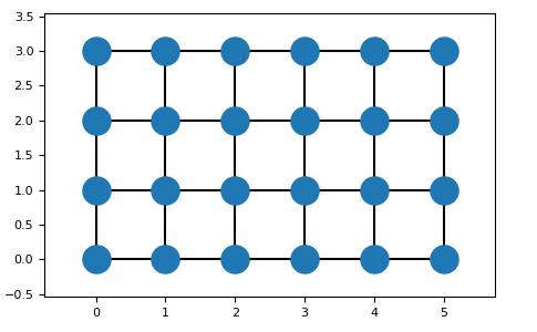
So far only the lattice structure has been configured. To actually construct a (finite) model of the lattice the model has to be built:

>>> latt.build(shape=(5, 3))

To view the built lattice the plot-method can be used:

>>> import matplotlib.pyplot as plt
>>> from lattpy import simple_square
>>> latt = simple_square()
>>> latt.build(shape=(5, 3))
>>> latt.plot()
>>> plt.show()

(png, pdf)

After configuring the lattice the attributes are available. Even without building a (finite) lattice structure all attributes can be computed on the fly for a given lattice vector, consisting of the translation vector n and the atom index alpha. For computing the (translated) atom positions the get_position method is used. Also, the neighbors and the vectors to these neighbors can be calculated. The dist_idx-parameter specifies the distance of the neighbors (0 for nearest neighbors, 1 for next nearest neighbors, …):

>>> latt.get_position(n=[0, 0], alpha=0)
[0. 0.]
>>> latt.get_neighbors([0, 0], alpha=0, distidx=0)
[[ 1  0  0]
 [ 0 -1  0]
 [-1  0  0]
 [ 0  1  0]]
>>> latt.get_neighbor_vectors(alpha=0, distidx=0)
[[ 1.  0.]
 [ 0. -1.]
 [-1.  0.]
 [ 0.  1.]]

Also, the reciprocal lattice vectors can be computed

>>> latt.reciprocal_vectors()
[[6.28318531 0.        ]
 [0.         6.28318531]]

or used to construct the reciprocal lattice:

>>> rlatt = latt.reciprocal_lattice()

The 1. Brillouin zone is the Wigner-Seitz cell of the reciprocal lattice:

>>> bz = rlatt.wigner_seitz_cell()

The 1.BZ can also be obtained by calling the explicit method of the direct lattice:

>>> bz = latt.brillouin_zone()

If the lattice has been built the necessary data is cached. The lattice sites of the structure then can be accessed by a simple index i. The syntax is the same as before, just without the get_ prefix:

>>> i = 2
>>>
>>> # Get position of the atom with index i=2
>>> positions = latt.position(i)
>>> # Get the atom indices of the nearest neighbors of the atom with index i=2
>>> neighbor_indices = latt.neighbors(i, distidx=0)
>>> # the nearest neighbors can also be found by calling (equivalent to dist_idx=0)
>>> neighbor_indices = latt.nearest_neighbors(i)